Basic Column Math
Some of the most basic things you probably do regularly in Excel or Google Sheets are to find column totals or averages. In Excel, you would need to type a short function like “=SUM(A1:A10)” to add up the values in a column. In R, we do the same thing but you can reference columns by name and there are more built in commands that make writing the functions easier.
Note that in R you can basically use the words “function” and “command” interchangeably. Technically, you run a command that performs a function, but since the function its performing is also the command name, they’re the same thing.
For example, if we wanted to find the total of all the prices in the price column, we would do sum(treats$price). If we wanted to find the average price of treats we would do mean(treats$price).
Here are those commands to run plus a few more. See if you can figure out what the new ones do. (And if not, just read below.)
If you are ever unsure what a command does, like maybe n() or sd(), you can see the documentation for the command by running the line ?command, where command is the name of the function you want to learn about. Try running this code to understand what n() does and then change it to find out what sd() does.
In RStudio, I usually run ?command in the console instead of the script because I don’t need that to be saved in my final script; it’s just a scratch paper thing.

Piping Data
In R, “piping” refers to passing the output of one function directly into another function, without needing to create intermediate variables. This makes code more readable and easier to follow. We do this using the %>% command. (You will see %>% in older R code and |> in newer R code. They do the same thing. Reed tends to be slow to new things, so I’m using %>% here.)
This means we can do something like x + y and without storing it as z, we can basically have a temporary z and “pipe” it to another command that will change it further and then show only the final output. .
We’ll use the unique() and distinct() commands to demonstrate. These commands do very similar things, but one uses %>% and the other doesn’t. First we’ll work without the pipe:
(Do you understand what it is doing? If not you can always run ?unique to find out.)
Now we’ll do the same thing using %>% and the function distinct(). To pipe to the function we say the name of the dataset, the pipe command, and then the other functions we would like to use on the intermediate output. In this example, the coding difference is trivial, but you will see the usefulness of piping on the next pages.
Note that with unique() you have to use the data$column format, but with distinct you can just say the column name; that’s one nice feature of pipes.
It is convention when using
%>%to always put the next bit of code on a new line; this just helps keep the code neat and easy to read.
Sorting Columns
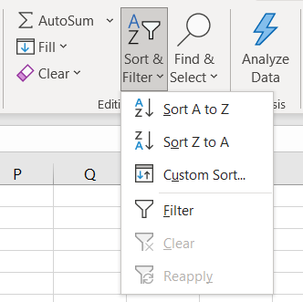
Another common thing you have probably done in Excel is sort the data by alphabetical or numerical order. In Excel, this is done via a point-and-click menu option, but in R you do the same thing directly with a line of code.
Here’s the Excel way:

And here’s the R way with the function arrange(). Note that we’re also using the pipe command here.
We can also use different options with arrange() to change the order of our sorting. Here we add the nested function desc() which is short for descending, so now the highest values will be displayed at the top.
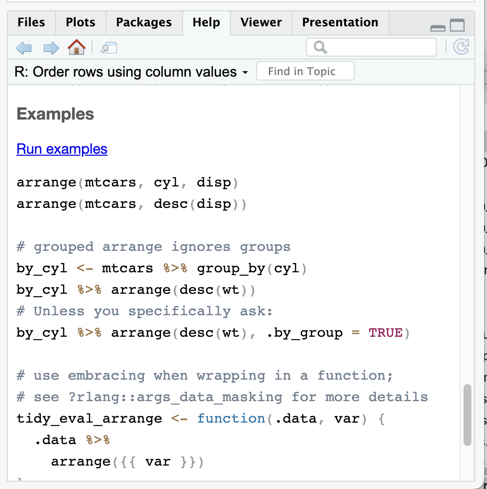
If you didn’t know about the desc() add on, one thing you could do is run ?arrange to see what other options arrange() has. The top of the Help section is often a bit jargon-y, but if you scroll to the bottom of the Help window, you can see examples that are more useful.
Here are the examples for arrange(). All of them use built in data, so you can run the examples to see what they do.
